Today we continued our work with proofs by induction. I’m gonna be honest, I am NOT a fan of induction! I’m hoping that eventually I’ll have an “ah-ha” moment where it clicks in my brain, but until that happens I’m struggling with understanding what exactly to use as a base case and how to prove that if  is true, then so is
  . We began class by learning how you can use a contrapositive approach when using induction. To demonstrate this, Casey wrote out the goal of “standard” induction and then the goal of “contrapositive” induction:
Standard

Contrapositive

We also learned that the contrapositive approach to induction is referred to as the proof by least counter-example method. I liked writing the goals out in this notation because while I don’t really understand how to make induction work, this helps give me a visual representation of what I am trying to do. I assuming that like the “normal” contrapositive approach to proofs, this one can only be used when we’re given an “if-then” statement.
We then moved on to discussing the Fundamental Theory of Arithmetic, which is arguably the most important proof we’ve learned to date. The theorem says that any number can be written as the product of two prime numbers. For example,  and
and  . In more math-y terms, this can be expressed as:

We can read about this on page 164 in our textbook, which I have done, but still don’t quite understand it, so I’m going to look at it more in the near future in the hopes I can understand it better. We were told before reading it that the three things we need to prove this are: (1) strong induction (2) cases and (3) proof by least counter-example.
We then went over a proof about cows that basically shows that the induction method could actually be complete bullshit.

The proof basically says that all cows are brown, which obviously isn’t true, but the proof makes a pretty convincing argument. It’s just a tad bit trippy. Instead of rewriting the proof just like we did it in class, I will replace the cows with something a little more exciting…LIGHTSABERS! In honor of my boy Obi-Wan, I am going to claim that all lightsabers are blue.
Proposition
All lightsabers are blue.
Proof
Base case: {one blue lightsaber}
Inductive step: Suppose whenever someone has a set of  lightsabers, that all
  are known.
WTS that in any set of  lightsabers, all lightsabers are blue.
Let  be any set with lightsabers.
Consider that 
By assumption this would mean that all lightsabers in  are blue.
Consider 


Thus, our hypothesis implies that the lightsabers in  are blue.
 is blue
 all lightsabers in are blue.
*****the base case could have been something like “the same color” instead of blue*****
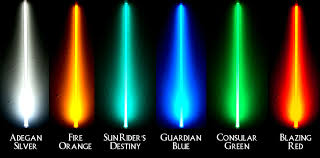
We know that this isn’t true because there are other options for lightsabers (purple, green, red,…) but the proof above is still a relatively solid proof. This is why some mathematicians are skeptical about using induction to prove things. However, I can see how induction is an important way to think about proofs even if I don’t yet fully understand it.
After this, we just spent the rest of class working on homework, which I didn’t really make much headway on. I plan on blogging more about this later, so in order to avoid repeating myself, that’ all for now.
Peace
Emily


![{A]=\text{the domain of f}\Rightarrow\forall{a}\in{A},f(a)\in{B}](https://s0.wp.com/latex.php?latex=%7BA%5D%3D%5Ctext%7Bthe+domain+of+f%7D%5CRightarrow%5Cforall%7Ba%7D%5Cin%7BA%7D%2Cf%28a%29%5Cin%7BB%7D&bg=ffffff&fg=444444&s=0&c=20201002)


 on a set
  can be used to partition
 ![\{[\mathrm{a}] : \mathrm{a}\in\mathrm{A}\} = \mathrm{A}/\sim](https://s0.wp.com/latex.php?latex=%5C%7B%5B%5Cmathrm%7Ba%7D%5D+%3A+%5Cmathrm%7Ba%7D%5Cin%5Cmathrm%7BA%7D%5C%7D+%3D+%5Cmathrm%7BA%7D%2F%5Csim&bg=ffffff&fg=444444&s=0&c=20201002) is a partition for
is a partition for ![\bigcup_{\mathrm{a}\in\mathrm{A}}[\mathrm{a}] = \mathrm{A}](https://s0.wp.com/latex.php?latex=%5Cbigcup_%7B%5Cmathrm%7Ba%7D%5Cin%5Cmathrm%7BA%7D%7D%5B%5Cmathrm%7Ba%7D%5D+%3D+%5Cmathrm%7BA%7D&bg=ffffff&fg=444444&s=0&c=20201002)
![\forall\mathrm{a}\in\mathrm{A},\mathrm{a}\in\[\mathrm{a}]\Rightarrow[\mathrm{a}]=\text{empty set}](https://s0.wp.com/latex.php?latex=%5Cforall%5Cmathrm%7Ba%7D%5Cin%5Cmathrm%7BA%7D%2C%5Cmathrm%7Ba%7D%5Cin%5C%5B%5Cmathrm%7Ba%7D%5D%5CRightarrow%5B%5Cmathrm%7Ba%7D%5D%3D%5Ctext%7Bempty+set%7D&bg=ffffff&fg=444444&s=0&c=20201002) .
.![[\mathrm{a}] \cap[\mathrm{b}]\neq\emptyset](https://s0.wp.com/latex.php?latex=%5B%5Cmathrm%7Ba%7D%5D+%5Ccap%5B%5Cmathrm%7Bb%7D%5D%5Cneq%5Cemptyset&bg=ffffff&fg=444444&s=0&c=20201002) . This means
. This means ![\exists\mathrm{x}\in\mathrm{A}, \mathrm{x}\in[\mathrm{a}]](https://s0.wp.com/latex.php?latex=%5Cexists%5Cmathrm%7Bx%7D%5Cin%5Cmathrm%7BA%7D%2C+%5Cmathrm%7Bx%7D%5Cin%5B%5Cmathrm%7Ba%7D%5D&bg=ffffff&fg=444444&s=0&c=20201002) and
and ![\mathrm{x}\in[\mathrm{b}]](https://s0.wp.com/latex.php?latex=%5Cmathrm%7Bx%7D%5Cin%5B%5Cmathrm%7Bb%7D%5D&bg=ffffff&fg=444444&s=0&c=20201002) . Hence,
. Hence,  the tells us that by symmetry we have
  which through transitivity implies that
  .
.![\mathrm{y}\in[\mathrm{a}]\Rightarrow\mathrm{y}~\mathrm{a}\Rightarrow\mathrm{y}~\mathrm{b}\Rightarrow\mathrm{y}\in[\mathrm{b}]](https://s0.wp.com/latex.php?latex=%5Cmathrm%7By%7D%5Cin%5B%5Cmathrm%7Ba%7D%5D%5CRightarrow%5Cmathrm%7By%7D%7E%5Cmathrm%7Ba%7D%5CRightarrow%5Cmathrm%7By%7D%7E%5Cmathrm%7Bb%7D%5CRightarrow%5Cmathrm%7By%7D%5Cin%5B%5Cmathrm%7Bb%7D%5D&bg=ffffff&fg=444444&s=0&c=20201002) . As a result,
. As a result, ![[\mathrm{a}]\subseteq[\mathrm{b} Now, let](https://s0.wp.com/latex.php?latex=%5B%5Cmathrm%7Ba%7D%5D%5Csubseteq%5B%5Cmathrm%7Bb%7D++++Now%2C+let+&bg=ffffff&fg=444444&s=0&c=20201002) latex \mathrm{z}\in[\mathrm{b}]\Rightarrow\mathrm{z}~\mathrm{b}$
latex \mathrm{z}\in[\mathrm{b}]\Rightarrow\mathrm{z}~\mathrm{b}$ (transitivity)
![\Rightarrow\mathrm{z}\in[\mathrm{a}]](https://s0.wp.com/latex.php?latex=%5CRightarrow%5Cmathrm%7Bz%7D%5Cin%5B%5Cmathrm%7Ba%7D%5D&bg=ffffff&fg=444444&s=0&c=20201002)
![\Rightarrow[\mathrm{b}]=[\mathrm{a}]](https://s0.wp.com/latex.php?latex=%5CRightarrow%5B%5Cmathrm%7Bb%7D%5D%3D%5B%5Cmathrm%7Ba%7D%5D&bg=ffffff&fg=444444&s=0&c=20201002)
![\bigcup_{\mathrm{a}\in\mathrm{A}}[\mathrm{a}]=\mathrm{A}](https://s0.wp.com/latex.php?latex=%5Cbigcup_%7B%5Cmathrm%7Ba%7D%5Cin%5Cmathrm%7BA%7D%7D%5B%5Cmathrm%7Ba%7D%5D%3D%5Cmathrm%7BA%7D&bg=ffffff&fg=444444&s=0&c=20201002) we will argue two implications:
we will argue two implications:![\bigcup_{\mathrm{a}\in\mathrm{A}}[\mathrm{a}]\subseteq\mathrm{A}](https://s0.wp.com/latex.php?latex=%5Cbigcup_%7B%5Cmathrm%7Ba%7D%5Cin%5Cmathrm%7BA%7D%7D%5B%5Cmathrm%7Ba%7D%5D%5Csubseteq%5Cmathrm%7BA%7D&bg=ffffff&fg=444444&s=0&c=20201002)

![\mathrm{x}\in\bigcup_{\mathrm{a}\in\mathrm{A}}[\mathrm{a}]](https://s0.wp.com/latex.php?latex=%5Cmathrm%7Bx%7D%5Cin%5Cbigcup_%7B%5Cmathrm%7Ba%7D%5Cin%5Cmathrm%7BA%7D%7D%5B%5Cmathrm%7Ba%7D%5D&bg=ffffff&fg=444444&s=0&c=20201002) . This means that
. This means that  for some
  . In essence,
 ![\mathrm{x}\in[\mathrm{a}]=\{\mathrm{w}\in\mathrm{A}:\mathrm{w}~\mathrm{a}\}](https://s0.wp.com/latex.php?latex=%5Cmathrm%7Bx%7D%5Cin%5B%5Cmathrm%7Ba%7D%5D%3D%5C%7B%5Cmathrm%7Bw%7D%5Cin%5Cmathrm%7BA%7D%3A%5Cmathrm%7Bw%7D%7E%5Cmathrm%7Ba%7D%5C%7D&bg=ffffff&fg=444444&s=0&c=20201002)

 . Since
 ![\mathrm{y}~\mathrm{y}\Rightarrow\mathrm{y}\in[\mathrm{y}]\Rightarrow\mathrm{y}\in\bigcup_{\mathrm{a}\in\mathrm{A}}[\mathrm{a}]](https://s0.wp.com/latex.php?latex=%5Cmathrm%7By%7D%7E%5Cmathrm%7By%7D%5CRightarrow%5Cmathrm%7By%7D%5Cin%5B%5Cmathrm%7By%7D%5D%5CRightarrow%5Cmathrm%7By%7D%5Cin%5Cbigcup_%7B%5Cmathrm%7Ba%7D%5Cin%5Cmathrm%7BA%7D%7D%5B%5Cmathrm%7Ba%7D%5D&bg=ffffff&fg=444444&s=0&c=20201002) .
. 

 is partitioned by
 ![\{[\text{ deg 0}], [\text{deg 1 }], \text{...}\}](https://s0.wp.com/latex.php?latex=%5C%7B%5B%5Ctext%7B+deg+0%7D%5D%2C+%5B%5Ctext%7Bdeg+1+%7D%5D%2C+%5Ctext%7B...%7D%5C%7D&bg=ffffff&fg=444444&s=0&c=20201002)
![\Rightarrow \mathrm{S} = \{ [2], [\mathrm{x}], [\mathrm{x}^{2}], \text{...}\}](https://s0.wp.com/latex.php?latex=%5CRightarrow+%5Cmathrm%7BS%7D+%3D+%5C%7B+%5B2%5D%2C+%5B%5Cmathrm%7Bx%7D%5D%2C+%5B%5Cmathrm%7Bx%7D%5E%7B2%7D%5D%2C+%5Ctext%7B...%7D%5C%7D&bg=ffffff&fg=444444&s=0&c=20201002)
![[2] + [\mathrm{x}] = [2 + \mathrm{x}]](https://s0.wp.com/latex.php?latex=%5B2%5D+%2B+%5B%5Cmathrm%7Bx%7D%5D+%3D+%5B2+%2B+%5Cmathrm%7Bx%7D%5D&bg=ffffff&fg=444444&s=0&c=20201002) which is degree equivalent with:
which is degree equivalent with:![[2] + [5\mathrm{x}] = [2 + 5\mathrm{x}]](https://s0.wp.com/latex.php?latex=%5B2%5D+%2B+%5B5%5Cmathrm%7Bx%7D%5D+%3D+%5B2+%2B+5%5Cmathrm%7Bx%7D%5D&bg=ffffff&fg=444444&s=0&c=20201002)
![\mathrm{A} = \mathbb{Z}, \mathrm{x}~\mathrm{y}\text{ if }\mathrm{x}\equiv\mathrm{y}\text{mod}{4}, \mathbb{Z}/ = \{[0], [1], [2], [3]\}](https://s0.wp.com/latex.php?latex=%5Cmathrm%7BA%7D+%3D+%5Cmathbb%7BZ%7D%2C+%5Cmathrm%7Bx%7D%7E%5Cmathrm%7By%7D%5Ctext%7B+if+%7D%5Cmathrm%7Bx%7D%5Cequiv%5Cmathrm%7By%7D%5Ctext%7Bmod%7D%7B4%7D%2C+%5Cmathbb%7BZ%7D%2F+%3D+%5C%7B%5B0%5D%2C+%5B1%5D%2C+%5B2%5D%2C+%5B3%5D%5C%7D&bg=ffffff&fg=444444&s=0&c=20201002)


![[\mathrm{a}] = \{\mathrm{x}\in\mathrm{A} : \mathrm{x} ~ \mathrm{a}\}](https://s0.wp.com/latex.php?latex=%5B%5Cmathrm%7Ba%7D%5D+%3D+%5C%7B%5Cmathrm%7Bx%7D%5Cin%5Cmathrm%7BA%7D+%3A+%5Cmathrm%7Bx%7D+%7E+%5Cmathrm%7Ba%7D%5C%7D&bg=ffffff&fg=444444&s=0&c=20201002)


 by:
by: means…
 means…
 means…
 are equal to the degree of
  *****
*****![[\mathrm{x}^{2}] = \{\text{all degree two polynomials\}](https://s0.wp.com/latex.php?latex=%5B%5Cmathrm%7Bx%7D%5E%7B2%7D%5D+%3D+%5C%7B%5Ctext%7Ball+degree+two+polynomials%5C%7D&bg=ffffff&fg=444444&s=0&c=20201002)
![[28] \cup [\mathrm{x}] \cup [\mathrm{x}^{2}] \cup [\mathrm{x}^{3}] \cup \text{...}](https://s0.wp.com/latex.php?latex=%5B28%5D+%5Ccup+%5B%5Cmathrm%7Bx%7D%5D+%5Ccup+%5B%5Cmathrm%7Bx%7D%5E%7B2%7D%5D+%5Ccup+%5B%5Cmathrm%7Bx%7D%5E%7B3%7D%5D+%5Ccup+%5Ctext%7B...%7D&bg=ffffff&fg=444444&s=0&c=20201002)

![[\mathrm{x}] : = \{\mathrm{a}\in\mathrm{A}: \mathrm{aRx}\subseteq\mathrm{A}\}](https://s0.wp.com/latex.php?latex=%5B%5Cmathrm%7Bx%7D%5D+%3A+%3D+%5C%7B%5Cmathrm%7Ba%7D%5Cin%5Cmathrm%7BA%7D%3A+%5Cmathrm%7BaRx%7D%5Csubseteq%5Cmathrm%7BA%7D%5C%7D&bg=ffffff&fg=444444&s=0&c=20201002)
![\mathrm{A} = \bigcup_{\mathrm{x}\in\mathrm{A}}=[\mathrm{x}]](https://s0.wp.com/latex.php?latex=%5Cmathrm%7BA%7D+%3D+%5Cbigcup_%7B%5Cmathrm%7Bx%7D%5Cin%5Cmathrm%7BA%7D%7D%3D%5B%5Cmathrm%7Bx%7D%5D&bg=ffffff&fg=444444&s=0&c=20201002)
![[\mathrm{x}]\cap[\mathrm{y}]\neq{0}](https://s0.wp.com/latex.php?latex=%5B%5Cmathrm%7Bx%7D%5D%5Ccap%5B%5Cmathrm%7By%7D%5D%5Cneq%7B0%7D&bg=ffffff&fg=444444&s=0&c=20201002)
![\Leftarrow\Rightarrow[\mathrm{x}] = [\mathrm{y}]](https://s0.wp.com/latex.php?latex=%5CLeftarrow%5CRightarrow%5B%5Cmathrm%7Bx%7D%5D+%3D+%5B%5Cmathrm%7By%7D%5D&bg=ffffff&fg=444444&s=0&c=20201002)


 was checked first.
 which I agree makes the most sense.
 . They’re called relations because the ordered pairs you get from the Cartesian Product relate
  and
and 

 relations, or “relations on

 .
. , then
  .
. , then
  .
.
 , which is the “most irrational number in terms of continued fractions.” While the Golden Ratio is cool and all, some people have gone a bit over board in claiming the Golden Ratio applies to a bunch of random crap. Criminal Minds even had an episode where the Golden Ratio and the Fibonacci Spiral were the key to solving a case. It’s a little ridiculous but I actually really like that show. Here’s a clip because you doesn’t like getting distracted by YouTube:
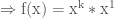
 that you’re just gonna continuously raise to some power to get another number:


![\displaystyle \left[\begin{array}{cc}1 & -1\\0 & 1\end{array}\right]^{\mathrm{n}}](https://s0.wp.com/latex.php?latex=%5Cdisplaystyle+%5Cleft%5B%5Cbegin%7Barray%7D%7Bcc%7D1+%26+-1%5C%5C0+%26+1%5Cend%7Barray%7D%5Cright%5D%5E%7B%5Cmathrm%7Bn%7D%7D&bg=ffffff&fg=444444&s=0&c=20201002) for all
for all 
![\displaystyle \left[\begin{array}{cc}1 & -\mathrm{n}\\0 & 1\end{array}\right]](https://s0.wp.com/latex.php?latex=%5Cdisplaystyle+%5Cleft%5B%5Cbegin%7Barray%7D%7Bcc%7D1+%26+-%5Cmathrm%7Bn%7D%5C%5C0+%26+1%5Cend%7Barray%7D%5Cright%5D&bg=ffffff&fg=444444&s=0&c=20201002) . We will attempt to verify this using proof by induction.
. We will attempt to verify this using proof by induction.
![\displaystyle \left[\begin{array}{cc}1 & -1\\0 & 1\end{array}\right]^{1} = \left[\begin{array}{cc}1 & -1\\0 & 1\end{array}\right]](https://s0.wp.com/latex.php?latex=%5Cdisplaystyle+%5Cleft%5B%5Cbegin%7Barray%7D%7Bcc%7D1+%26+-1%5C%5C0+%26+1%5Cend%7Barray%7D%5Cright%5D%5E%7B1%7D+%3D+%5Cleft%5B%5Cbegin%7Barray%7D%7Bcc%7D1+%26+-1%5C%5C0+%26+1%5Cend%7Barray%7D%5Cright%5D&bg=ffffff&fg=444444&s=0&c=20201002) , which supports our formula.
, which supports our formula.![\mathrm{S}_{\mathrm{k}} = \displaystyle \left[\begin{array}{cc}1 & -1\\0 & 1\end{array}\right]^{k} = \left[\begin{array}{cc}1 & -\mathrm{k}\\0 & 1\end{array}\right]](https://s0.wp.com/latex.php?latex=%5Cmathrm%7BS%7D_%7B%5Cmathrm%7Bk%7D%7D+%3D+%5Cdisplaystyle+%5Cleft%5B%5Cbegin%7Barray%7D%7Bcc%7D1+%26+-1%5C%5C0+%26+1%5Cend%7Barray%7D%5Cright%5D%5E%7Bk%7D+%3D+%5Cleft%5B%5Cbegin%7Barray%7D%7Bcc%7D1+%26+-%5Cmathrm%7Bk%7D%5C%5C0+%26+1%5Cend%7Barray%7D%5Cright%5D&bg=ffffff&fg=444444&s=0&c=20201002)
![\mathrm{S}_{\mathrm{k}+1} = \displaystyle \left[\begin{array}{cc}1 & -1\\0 & 1\end{array}\right]^{\mathrm{k}+1} = \displaystyle \left[\begin{array}{cc}1 & -(\mathrm{k}+1)\\0 & 1\end{array}\right]](https://s0.wp.com/latex.php?latex=%5Cmathrm%7BS%7D_%7B%5Cmathrm%7Bk%7D%2B1%7D+%3D+%5Cdisplaystyle+%5Cleft%5B%5Cbegin%7Barray%7D%7Bcc%7D1+%26+-1%5C%5C0+%26+1%5Cend%7Barray%7D%5Cright%5D%5E%7B%5Cmathrm%7Bk%7D%2B1%7D+%3D+%5Cdisplaystyle+%5Cleft%5B%5Cbegin%7Barray%7D%7Bcc%7D1+%26+-%28%5Cmathrm%7Bk%7D%2B1%29%5C%5C0+%26+1%5Cend%7Barray%7D%5Cright%5D&bg=ffffff&fg=444444&s=0&c=20201002)
![\mathrm{S}_{\mathrm{k}+1} = \displaystyle \left[\begin{array}{cc}1 & -1\\0 & 1\end{array}\right]^{\mathrm{k}} * \displaystyle \left[\begin{array}{cc}1 & -1\\0 & 1\end{array}\right]^{1}](https://s0.wp.com/latex.php?latex=%5Cmathrm%7BS%7D_%7B%5Cmathrm%7Bk%7D%2B1%7D+%3D+%5Cdisplaystyle+%5Cleft%5B%5Cbegin%7Barray%7D%7Bcc%7D1+%26+-1%5C%5C0+%26+1%5Cend%7Barray%7D%5Cright%5D%5E%7B%5Cmathrm%7Bk%7D%7D+%2A+%5Cdisplaystyle+%5Cleft%5B%5Cbegin%7Barray%7D%7Bcc%7D1+%26+-1%5C%5C0+%26+1%5Cend%7Barray%7D%5Cright%5D%5E%7B1%7D&bg=ffffff&fg=444444&s=0&c=20201002)
![\mathrm{S}_{\mathrm{k}+1} = \displaystyle \left[\begin{array}{cc}1 & -(\mathrm{k}+1)\\0 & 1\end{array}\right]](https://s0.wp.com/latex.php?latex=%5Cmathrm%7BS%7D_%7B%5Cmathrm%7Bk%7D%2B1%7D+%3D+%5Cdisplaystyle+%5Cleft%5B%5Cbegin%7Barray%7D%7Bcc%7D1+%26+-%28%5Cmathrm%7Bk%7D%2B1%29%5C%5C0+%26+1%5Cend%7Barray%7D%5Cright%5D&bg=ffffff&fg=444444&s=0&c=20201002) , which is what we wanted.
, which is what we wanted. our formula
  ) is true and that
  .
. then
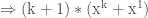
then  and based on our understanding of exponents we know that this can be rewritten as
  and using induction we know that in this case the derivative is still 1.

 , the derivative is also 1.
 then
then  .
.
 we can use the product rule to find the derivative. Recall that based on our assumptions we know that both
  and
and  are in fact true and we know their derivatives.
 and let


 , which is what we WTS.


